Divide & Conquer

Introduction

Divide and conquer is a basic but powerful technique that is widely used in many algorithms. As you might speculate from its name, the principle of divide and conquer is to recursively divide a complicated problem into a few simple sub-problems of the same type (divide), until they become simple enough and we can solve them quickly (conquer); finally we will combine the sub-result to get the final result. Thus, we’ll usually use recursion when we want to use the divide and conquer algorithm.

Merge Sort Algorithm

Merge Sort is a classic divide and conquer algorithm; let’s look at its program specification:

Algorithm: merge sort
input: an array arr[] of comparable element
output: sorted version of the input array, ascending

In merge sort, we’ll apply the divide and conquer idea. Divide: we’ll recursively divide the array into two-parts until we can not divide anymore. At this time, all sub-arrays contains only one element; therefore, they can be considered as sorted array. Conquer: now, the question becomes how to merge two sorted arrays (left-half and right-half) into a single sorted array; this is easy and can be done with O(n) time. To make it clear, we can have another function called merge:

Algorithm: merge
input: two sorted array arr1[], arr2[] of comparable element
output: one sorted array, ascending 

And we can write the pseudocode for merge sort:

arr[] mergesort(arr[]) {
  if (the length of arr[] is 1)
    return arr[]
  left[] <-- copy the left half of arr[]
  right[] <-- copy the right half of arr[]
  left[] = mergesort(left[])
  right[] = mergesort(right[])
  return merge(left[], right[])
}

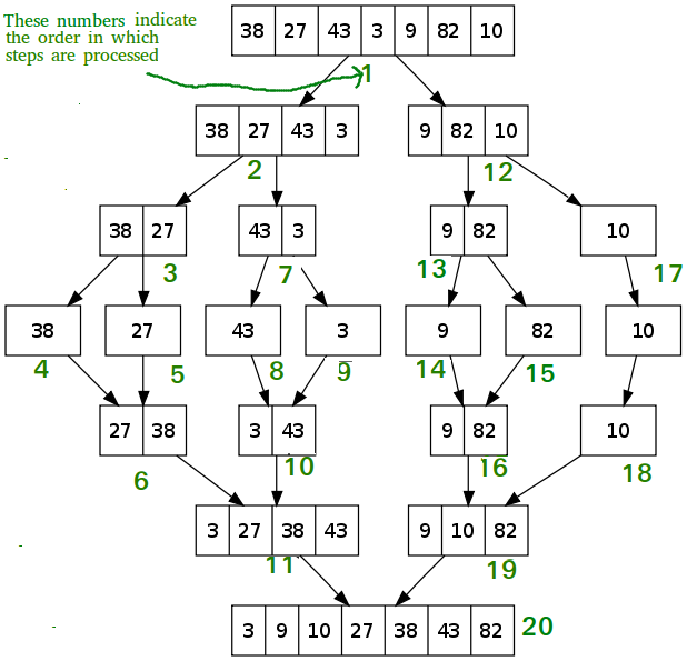
Here is an concrete example from GeeksforGeeks with every step shown in order, assuming our input array is [38, 27, 43, 3, 9, 82,10]:

Algorithm analyze

Time Complexity: Let n be the number of element in our input array. Since we are recursively dividing the array into two-part, the height of the tree will be 2log(n). Consider every level before merging (the upper log(n) levels), all we do is splitting the current array into left-half and right-half, which can be done with O(n) time. Consider every level after merging (the lower log(n) levels), what we do is merging two sorted arrays, this can be done with two pointers within O(n) time. To sum all these up, the total time complexity is O(n*logn)

Space Complexity: we will need O(n) extra space to store the left-half and right-half sub-arrays we created at any time. If we also want to consider the space used by recursive calls, we need to add extra O(logn) space for the stack frames. Thus, the total space complexity is O(n) +O(logn)

Conclusion

Similar to merge sort, other classic algorithms like binary search, quick sort, closest pairs in 2-d space also use the idea of divide & conquer algorithm. Two things need to be noticed here: 1. the subproblems are easier to solve than the current problem; in other words, dividing need to reduce the difficulty of the problem. 2. The subproblems need to be in the same format so that they can be solved similarly and efficiently, which will be time-saving.

Interestingly, what if the same subproblem occurs multiple times during division? In that case, another algorithm, dynamic programming, similar to divide & conquer, can be applied. We’d like to remember the state/result of the subproblem and only solve the same subproblem once instead of multiple times.

Have fun!